Gaussian Process Examples
This notebook demonstrates how to use tmg_hmc to sample from constrained Gaussian processes (GPs). A GP is a distribution over functions that places a multivariate Gaussian distribution over function values at a finite set of points. By imposing linear constraints on those function values (or their derivatives), we can sample GP realizations that satisfy shape constraints such as boundedness, monotonicity, or convexity.
The key property enabling this is that derivative information can be incorporated into the GP by augmenting the covariance matrix with cross-covariances between function values and derivatives. This is possible because linear functions (including derivatives) of a GP are themselves GPs.
Setup
Install notebook dependencies if needed:
pip install tmg_hmc[examples]
[1]:
import numpy as np
import matplotlib.pyplot as plt
from tmg_hmc import TMGSampler

# Set seed for reproducibility
np.random.seed(42)
Define Kernels
We use a squared exponential (RBF) kernel with length scale \(\ell\) and variance \(\sigma^2\):
To enforce derivative constraints, we also need the cross-covariances between function values and their first and second derivatives. These are obtained by differentiating the kernel analytically:
\(\text{Cov}(f(x_1), f'(x_2)) = \frac{\partial k}{\partial x_2}\)
\(\text{Cov}(f'(x_1), f'(x_2)) = \frac{\partial^2 k}{\partial x_1 \partial x_2}\)
\(\text{Cov}(f(x_1), f''(x_2)) = \frac{\partial^2 k}{\partial x_2^2}\)
\(\text{Cov}(f''(x_1), f''(x_2)) = \frac{\partial^4 k}{\partial x_1^2 \partial x_2^2}\)
[2]:
class SQExponentialKernel:
    def __init__(self, length_scale=1.0, variance=1.0):
        self.length_scale = length_scale
        self.variance = variance

    def __call__(self, x1, x2, cov_type="x_x"):
        if cov_type == "x_x":
            return self.cov_x_x(x1, x2)
        elif cov_type == "x_dx":
            return self.cov_x_dx(x1, x2)
        elif cov_type == "dx_x":
            return self.cov_dx_x(x1, x2)
        elif cov_type == "dx_dx":
            return self.cov_dx_dx(x1, x2)
        elif cov_type == "x_d2x":
            return self.cov_x_d2x(x1, x2)
        elif cov_type == "d2x_x":
            return self.cov_d2x_x(x1, x2)
        elif cov_type == "d2x_d2x":
            return self.cov_d2x_d2x(x1, x2)
        else:
            raise ValueError(f"Unknown covariance type: {cov_type}")

    def cov_x_x(self, x1, x2):
        """Covariance between function values: k(x1, x2)"""
        x1 = np.atleast_1d(x1).flatten()
        x2 = np.atleast_1d(x2).flatten()
        sqdist = (x1[:, None] - x2[None, :]) ** 2
        return self.variance * np.exp(-0.5 / self.length_scale**2 * sqdist)

    def cov_x_dx(self, x1, x2):
        """Covariance between function and first derivative: (x1 - x2) / l^2 * k(x1, x2)"""
        x1 = np.atleast_1d(x1).flatten()
        x2 = np.atleast_1d(x2).flatten()
        K = self.cov_x_x(x1, x2)
        diff = x1[:, None] - x2[None, :]
        return (diff / self.length_scale**2) * K

    def cov_dx_x(self, x1, x2):
        """Covariance between first derivative and function: -(x1 - x2) / l^2 * k(x1, x2)"""
        return -self.cov_x_dx(x1, x2)

    def cov_dx_dx(self, x1, x2):
        """Covariance between first derivatives: k(x1, x2) * [1/l^2 - (x1 - x2)^2/l^4]"""
        x1 = np.atleast_1d(x1).flatten()
        x2 = np.atleast_1d(x2).flatten()
        K = self.cov_x_x(x1, x2)
        diff = x1[:, None] - x2[None, :]
        return K * ((1 / self.length_scale**2) - (diff**2 / self.length_scale**4))

    def cov_x_d2x(self, x1, x2):
        """Covariance between function and second derivative: k(x1, x2) * [(x1-x2)^2/l^4 - 1/l^2]"""
        x1 = np.atleast_1d(x1).flatten()
        x2 = np.atleast_1d(x2).flatten()
        K = self.cov_x_x(x1, x2)
        diff = x1[:, None] - x2[None, :]
        return K * ((diff**2 / self.length_scale**4) - (1 / self.length_scale**2))

    def cov_d2x_x(self, x1, x2):
        """Covariance between second derivative and function (symmetric)"""
        return self.cov_x_d2x(x1, x2)

    def cov_d2x_d2x(self, x1, x2):
        """Covariance between second derivatives: k(x1,x2) * [3/l^4 - 6(x1-x2)^2/l^6 + (x1-x2)^4/l^8]"""
        x1 = np.atleast_1d(x1).flatten()
        x2 = np.atleast_1d(x2).flatten()
        K = self.cov_x_x(x1, x2)
        diff = x1[:, None] - x2[None, :]
        diff2 = diff**2
        diff4 = diff**4
        l4 = self.length_scale**4
        l6 = self.length_scale**6
        l8 = self.length_scale**8
        return K * (3 / l4 - 6 * diff2 / l6 + diff4 / l8)
Bounded GP
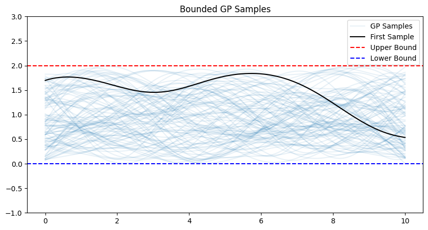
Here we sample GP realizations constrained to lie within a band \([l, u]\) at every point. This is achieved by adding two linear constraints per grid point \(x_i\):
\(f(x_i) \leq u\) written as \(-e_i^\top f + u \geq 0\)
\(f(x_i) \geq l\) written as \(e_i^\top f - l \geq 0\)
where \(e_i\) is the \(i\)-th standard basis vector. The covariance matrix is just the standard GP kernel evaluated at the grid points — no derivative augmentation is needed here.
[3]:
n = 100
x = np.linspace(0, 10, n)
kernel = SQExponentialKernel(length_scale=2.0, variance=2.0)
K = kernel(x, x, cov_type="x_x")

sampler = TMGSampler(mu=np.zeros((n, 1)), Sigma=K)

upper_bound = 2
lower_bound = 0
# Add constraints for each gridpoint: lower_bound <= f(x_i) <= upper_bound
for i in range(n):
    f = np.zeros((n, 1))
    f[i] = 1
    # f(x_i) <= upper_bound: -f(x_i) + upper_bound >= 0
    sampler.add_constraint(f=-f, c=upper_bound)
    # f(x_i) >= lower_bound: f(x_i) - lower_bound >= 0
    sampler.add_constraint(f=f, c=-lower_bound)

x0 = np.ones((n, 1)) * (upper_bound + lower_bound) / 2
samples = sampler.sample(x0, n_samples=100, burn_in=100)
[4]:
fig, ax = plt.subplots(1, 1, figsize=(10, 5))
ax.plot(x, samples[:-1].T, color="C0", alpha=0.1)
ax.plot(x, samples[-1], color="C0", alpha=0.1, label="GP Samples")
ax.plot(x, samples[0], color="black", label="First Sample")
ax.set_title("Bounded GP Samples")
ax.set_ylim(lower_bound - 1, upper_bound + 1)
ax.axhline(upper_bound, color="red", linestyle="--", label="Upper Bound")
ax.axhline(lower_bound, color="blue", linestyle="--", label="Lower Bound")
ax.legend()
plt.show()
Monotone GP
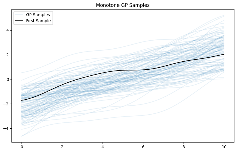
To sample monotonically non-decreasing GP realizations, we constrain the first derivative to be non-negative at every grid point: \(f'(x_i) \geq 0\).
To do this we augment the state vector to include both function values and derivative values: \(\mathbf{z} = (f(x_1), \ldots, f(x_n), f'(x_1), \ldots, f'(x_n))^\top\). The joint covariance matrix of this augmented vector is built using the kernel cross-covariances defined above.
The monotonicity constraint \(f'(x_i) \geq 0\) is then a linear constraint on the \((n+i)\)-th component of \(\mathbf{z}\).
[5]:
n = 100
x = np.linspace(0, 10, n)
kernel = SQExponentialKernel(length_scale=2.0, variance=2.0)

# Build augmented covariance matrix over [f(x), f'(x)]
K = np.block(
    [
        [kernel(x, x, cov_type="x_x"), kernel(x, x, cov_type="x_dx")],
        [kernel(x, x, cov_type="dx_x"), kernel(x, x, cov_type="dx_dx")],
    ]
)

sampler = TMGSampler(mu=np.zeros((2 * n, 1)), Sigma=K)

# Constrain f'(x_i) >= 0 for each grid point
# The derivative values occupy indices n, n+1, ..., 2n-1
for i in range(n):
    f = np.zeros((2 * n, 1))
    f[n + i] = 1
    sampler.add_constraint(f=f, c=0)

x0 = np.ones((2 * n, 1))
x0[:n] *= 0.0

samples = sampler.sample(x0, n_samples=100, burn_in=100)
[6]:
fig, ax = plt.subplots(figsize=(10, 6))
# Plot only the function values (first n components)
ax.plot(x, samples[:-1, :n].T, color="C0", alpha=0.1)
ax.plot(x, samples[-1, :n], color="C0", alpha=0.1, label="GP Samples")
ax.plot(x, samples[0, :n], color="black", label="First Sample")
ax.set_title("Monotone GP Samples")
ax.legend()
plt.show()
Convex GP
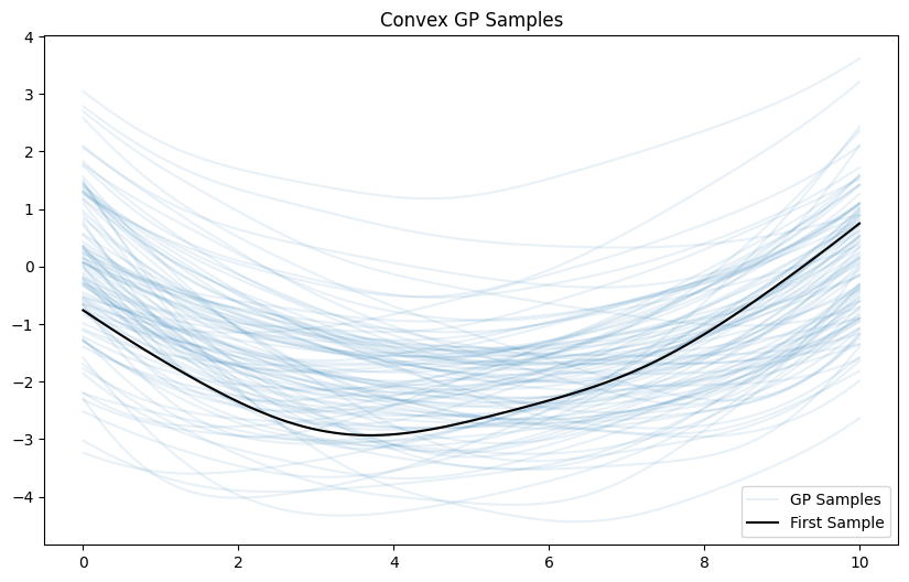
To sample convex GP realizations, we constrain the second derivative to be non-negative at every grid point: \(f''(x_i) \geq 0\).
The setup is analogous to the monotone case, but now we augment the state vector with second derivative values: \(\mathbf{z} = (f(x_1), \ldots, f(x_n), f''(x_1), \ldots, f''(x_n))^\top\). The joint covariance matrix is built using the function-value/second-derivative cross-covariances.
The convexity constraint \(f''(x_i) \geq 0\) is again a linear constraint on the \((n+i)\)-th component of \(\mathbf{z}\).
[7]:
n = 100
x = np.linspace(0, 10, n)
kernel = SQExponentialKernel(length_scale=2.0, variance=2.0)

# Build augmented covariance matrix over [f(x), f''(x)]
K = np.block(
    [
        [kernel(x, x, cov_type="x_x"), kernel(x, x, cov_type="x_d2x")],
        [kernel(x, x, cov_type="d2x_x"), kernel(x, x, cov_type="d2x_d2x")],
    ]
)

sampler = TMGSampler(mu=np.zeros((2 * n, 1)), Sigma=K)

# Constrain f''(x_i) >= 0 for each grid point
# The second derivative values occupy indices n, n+1, ..., 2n-1
for i in range(n):
    f = np.zeros((2 * n, 1))
    f[n + i] = 1
    sampler.add_constraint(f=f, c=0)

x0 = np.ones((2 * n, 1))
x0[:n] *= 0.0

samples = sampler.sample(x0, n_samples=100, burn_in=100)
[8]:
fig, ax = plt.subplots(figsize=(10, 6))
# Plot only the function values (first n components)
ax.plot(x, samples[:-1, :n].T, color="C0", alpha=0.1)
ax.plot(x, samples[-1, :n], color="C0", alpha=0.1, label="GP Samples")
ax.plot(x, samples[0, :n], color="black", label="First Sample")
ax.set_title("Convex GP Samples")
ax.legend()
plt.show()