Single Constraint Examples

This notebook demonstrates how to use tmg_hmc to sample from truncated multivariate Gaussians with a single constraint. Constraints are specified in the original space in the general form:

\[\mathbf{x}^\top A \mathbf{x} + \mathbf{f}^\top \mathbf{x} + c \geq 0\]

Internally, the sampler transforms the constraint to the standardized space \(\mathbf{y} = S^{-1}(\mathbf{x} - \boldsymbol{\mu})\) where \(S = \Sigma^{1/2}\), yielding:

\[\mathbf{y}^\top \tilde{A} \mathbf{y} + \tilde{\mathbf{f}}^\top \mathbf{y} + \tilde{c} \geq 0\]

where \(\tilde{A} = SAS\), \(\tilde{\mathbf{f}} = 2SA\boldsymbol{\mu} + S\mathbf{f}\), and \(\tilde{c} = \boldsymbol{\mu}^\top A \boldsymbol{\mu} + \mathbf{f}^\top \boldsymbol{\mu} + c\). The constraint type is then inferred based on which terms are non-zero in the transformed space:

• If \(\tilde{A} = 0\): a linear constraint \(\tilde{\mathbf{f}}^\top \mathbf{y} + \tilde{c} \geq 0\)

• If \(\tilde{A} \neq 0\) and \(\tilde{\mathbf{f}} = 0\): a simple quadratic constraint \(\mathbf{y}^\top \tilde{A} \mathbf{y} + \tilde{c} \geq 0\)

• If \(\tilde{A} \neq 0\) and \(\tilde{\mathbf{f}} \neq 0\): a full quadratic constraint

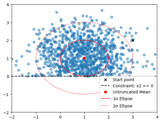
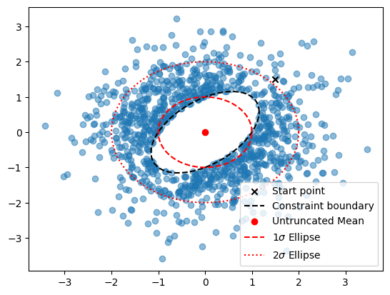
To further illustrate the effect of the truncations, we plot the untruncated mean and 1 and 2 \(\sigma\) ellipsoids of the untruncated Gaussian in red.

Setup

Install notebook dependencies if needed:

pip install tmg_hmc[examples]

from tmg_hmc import TMGSampler
import matplotlib.pyplot as plt
import numpy as np
import scipy as sp

# Set seed for reproducibility
np.random.seed(42)

Positivity (Linear Constraint)

We sample from \(\mathcal{N}([1, 1]^\top, I)\) constrained to \(x_2 \geq 0\). The constraint is specified with \(A = 0\), \(\mathbf{f} = [0, 1]^\top\), \(c = 0\).

With \(\boldsymbol{\mu} = [1,1]^\top\) and \(S = I\), the transformed constraint parameters are:

\[\tilde{A} = SAS = 0\]

\[\tilde{\mathbf{f}} = 2SA\boldsymbol{\mu} + S\mathbf{f} = \mathbf{0} + [0,1]^\top = [0,1]^\top\]

\[\tilde{c} = \boldsymbol{\mu}^\top A\boldsymbol{\mu} + \mathbf{f}^\top\boldsymbol{\mu} + c = 0 + 1 + 0 = 1\]

The transformed constraint is \(y_2 + 1 \geq 0\), i.e. \(y_2 \geq -1\). Since \(\tilde{A} = 0\), the sampler infers a LinearConstraint.

np.random.seed(0)
# N([1, 1], I) with x2 >= 0
mu = np.array([1.0, 1.0]).reshape(-1, 1)
sigma = np.eye(2)
sampler = TMGSampler(mu, sigma)

# Add positivity constraint: f^T x + c >= 0
# f = [0, 1], c = 0  =>  x2 >= 0
f = np.array([[0.0, 1.0]])
c = 0
sampler.add_constraint(f=f, c=c)
print(
    type(sampler.constraints[0])
)  # Constraint type is inferred after transforming to standardized space

<class 'tmg_hmc.constraints.linear.LinearConstraint'>

# Initialize at a point satisfying the constraint
x0 = np.array([3.0, 2.0]).reshape(-1, 1)
samples = sampler.sample(x0, n_samples=1000, burn_in=1000)

fig, ax = plt.subplots()
ax.scatter(samples[:, 0], samples[:, 1], alpha=0.5)
ax.scatter(x0[0], x0[1], color="k", marker="x", label="Start point")
ax.plot([-2, 4], [0, 0], "k--", label="Constraint: x2 >= 0")
ax.scatter(mu[0], mu[1], color="red", label="Untruncated Mean")
theta = np.linspace(0, 2 * np.pi, 100)
ellipse = np.array(
    [mu + sigma @ np.array([np.cos(t), np.sin(t)]).reshape(-1, 1) for t in theta]
)
ax.plot(
    ellipse[:, 0],
    ellipse[:, 1],
    color="red",
    linestyle="--",
    label=r"1$\sigma$ Ellipse",
)
ellipse2 = np.array(
    [mu + 2 * sigma @ np.array([np.cos(t), np.sin(t)]).reshape(-1, 1) for t in theta]
)
ax.plot(
    ellipse2[:, 0],
    ellipse2[:, 1],
    color="red",
    linestyle=":",
    label=r"2$\sigma$ Ellipse",
)
ax.set_ylim([-2, 4])
ax.set_xlim([-2, 4])
ax.legend()
plt.show()

Bounded Magnitude (Simple Quadratic Constraint)

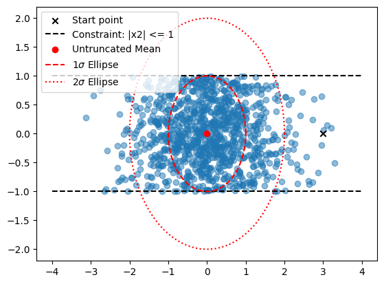
We sample from \(\mathcal{N}(\mathbf{0}, I)\) constrained to \(|x_2| \leq 1\) which is equivalent to \(x_2^2 \leq 1\). The constraint is specified with:

\[\begin{split}A = \begin{pmatrix} 0 & 0 \\ 0 & -1 \end{pmatrix}, \quad \mathbf{f} = \mathbf{0}, \quad c = 1\end{split}\]

With \(\boldsymbol{\mu} = \mathbf{0}\) and \(S = I\), the transformed constraint parameters are:

\[\begin{split}\tilde{A} = SAS = A = \begin{pmatrix} 0 & 0 \\ 0 & -1 \end{pmatrix}\end{split}\]

\[\tilde{\mathbf{f}} = 2SA\boldsymbol{\mu} + S\mathbf{f} = \mathbf{0}\]

\[\tilde{c} = \boldsymbol{\mu}^\top A\boldsymbol{\mu} + \mathbf{f}^\top\boldsymbol{\mu} + c = 0 + 0 + 1 = 1\]

The transformed constraint is \(-y_2^2 + 1 \geq 0\), i.e. \(|y_2| \leq 1\). Since \(\tilde{A} \neq 0\) and \(\tilde{\mathbf{f}} = 0\), the sampler infers a SimpleQuadraticConstraint.

mu = np.array([0.0, 0.0]).reshape(-1, 1)
sigma = np.eye(2)

# Constraint: -x2^2 + 1 >= 0  =>  |x2| <= 1
A = np.array([[0.0, 0.0], [0.0, -1.0]])
c = 1
sampler = TMGSampler(mu, sigma)
sampler.add_constraint(A=A, c=c)
print(
    type(sampler.constraints[0])
)  # Constraint type is inferred after transforming to standardized space

<class 'tmg_hmc.constraints.quadratic.SimpleQuadraticConstraint'>

x0 = np.array([3.0, 0.0]).reshape(-1, 1)
samples = sampler.sample(x0, n_samples=1000, burn_in=1000)

fig, ax = plt.subplots()
ax.scatter(samples[:, 0], samples[:, 1], alpha=0.5)
ax.scatter(x0[0], x0[1], color="k", marker="x", label="Start point")
ax.plot([-4, 4], [1, 1], "k--", label="Constraint: |x2| <= 1")
ax.plot([-4, 4], [-1, -1], "k--")
ax.scatter(mu[0], mu[1], color="red", label="Untruncated Mean")
theta = np.linspace(0, 2 * np.pi, 100)
ellipse = np.array(
    [mu + sigma @ np.array([np.cos(t), np.sin(t)]).reshape(-1, 1) for t in theta]
)
ax.plot(
    ellipse[:, 0],
    ellipse[:, 1],
    color="red",
    linestyle="--",
    label=r"1$\sigma$ Ellipse",
)
ellipse2 = np.array(
    [mu + 2 * sigma @ np.array([np.cos(t), np.sin(t)]).reshape(-1, 1) for t in theta]
)
ax.plot(
    ellipse2[:, 0],
    ellipse2[:, 1],
    color="red",
    linestyle=":",
    label=r"2$\sigma$ Ellipse",
)
ax.legend()
plt.show()

Bounded Inside Ellipsoid (Simple Quadratic Constraint)

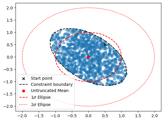
We sample from \(\mathcal{N}(\mathbf{0}, I)\) constrained to lie inside the ellipse \(x_1^2 + x_1 x_2 + x_2^2 \leq 1\). The constraint is specified with:

\[\begin{split}A = -\begin{pmatrix} 1 & 0.5 \\ 0.5 & 1 \end{pmatrix}, \quad \mathbf{f} = \mathbf{0}, \quad c = 1\end{split}\]

With \(\boldsymbol{\mu} = \mathbf{0}\) and \(S = I\), the transformed constraint parameters are:

\[\begin{split}\tilde{A} = SAS = A = -\begin{pmatrix} 1 & 0.5 \\ 0.5 & 1 \end{pmatrix}\end{split}\]

\[\tilde{\mathbf{f}} = 2SA\boldsymbol{\mu} + S\mathbf{f} = \mathbf{0}\]

\[\tilde{c} = \boldsymbol{\mu}^\top A\boldsymbol{\mu} + \mathbf{f}^\top\boldsymbol{\mu} + c = 0 + 0 + 1 = 1\]

The transformed constraint is \(-(y_1^2 + y_1 y_2 + y_2^2) + 1 \geq 0\), i.e. \(y_1^2 + y_1 y_2 + y_2^2 \leq 1\). Since \(\tilde{A} \neq 0\) and \(\tilde{\mathbf{f}} = 0\), the sampler infers a SimpleQuadraticConstraint.

mu = np.array([0.0, 0.0]).reshape(-1, 1)
sigma = np.eye(2)
sampler = TMGSampler(mu, sigma)

# Constraint: -(x1^2 + x1*x2 + x2^2) + 1 >= 0  =>  x1^2 + x1*x2 + x2^2 <= 1
A = -np.array([[1, 0.5], [0.5, 1]])
c = 1
sampler.add_constraint(A=A, c=c)
x0 = np.array([0.5, 0.5]).reshape(-1, 1)
samples = sampler.sample(x0, 1000, 100)

fig, ax = plt.subplots()
ax.scatter(samples[:, 0], samples[:, 1], alpha=0.5)
ax.scatter(x0[0], x0[1], color="k", marker="x", label="Start point")
theta = np.linspace(0, 2 * np.pi, 100)
sqA = sp.linalg.cholesky(np.linalg.inv(-A))
ellipse = np.array(
    [sqA.T @ np.array([np.cos(t), np.sin(t)]).reshape(-1, 1) for t in theta]
)
ax.plot(ellipse[:, 0], ellipse[:, 1], "k--", label="Constraint boundary")
ax.scatter(mu[0], mu[1], color="red", label="Untruncated Mean")
ellipse = np.array(
    [mu + sigma @ np.array([np.cos(t), np.sin(t)]).reshape(-1, 1) for t in theta]
)
ax.plot(
    ellipse[:, 0],
    ellipse[:, 1],
    color="red",
    linestyle="--",
    label=r"1$\sigma$ Ellipse",
)
ellipse2 = np.array(
    [mu + 2 * sigma @ np.array([np.cos(t), np.sin(t)]).reshape(-1, 1) for t in theta]
)
ax.plot(
    ellipse2[:, 0],
    ellipse2[:, 1],
    color="red",
    linestyle=":",
    label=r"2$\sigma$ Ellipse",
)
ax.legend()
plt.show()

Bounded Outside Ellipsoid (Simple Quadratic Constraint)

We sample from \(\mathcal{N}(\mathbf{0}, I)\) constrained to lie outside the ellipse \(x_1^2 - x_1 x_2 + x_2^2 \geq 1\). The constraint is specified with:

\[\begin{split}A = \begin{pmatrix} 1 & -0.5 \\ -0.5 & 1 \end{pmatrix}, \quad \mathbf{f} = \mathbf{0}, \quad c = -1\end{split}\]

With \(\boldsymbol{\mu} = \mathbf{0}\) and \(S = I\), the transformed constraint parameters are:

\[\begin{split}\tilde{A} = SAS = A = \begin{pmatrix} 1 & -0.5 \\ -0.5 & 1 \end{pmatrix}\end{split}\]

\[\tilde{\mathbf{f}} = 2SA\boldsymbol{\mu} + S\mathbf{f} = \mathbf{0}\]

\[\tilde{c} = \boldsymbol{\mu}^\top A\boldsymbol{\mu} + \mathbf{f}^\top\boldsymbol{\mu} + c = 0 + 0 - 1 = -1\]

The transformed constraint is \(y_1^2 - y_1 y_2 + y_2^2 - 1 \geq 0\), i.e. \(y_1^2 - y_1 y_2 + y_2^2 \geq 1\). Since \(\tilde{A} \neq 0\) and \(\tilde{\mathbf{f}} = 0\), the sampler infers a SimpleQuadraticConstraint.

mu = np.array([0.0, 0.0]).reshape(-1, 1)
sigma = np.eye(2)
sampler = TMGSampler(mu, sigma)

# Constraint: x1^2 - x1*x2 + x2^2 - 1 >= 0  =>  outside the ellipse
A = np.array([[1, -0.5], [-0.5, 1]])
c = -1
sampler.add_constraint(A=A, c=c)
x0 = np.array([1.5, 1.5]).reshape(-1, 1)
samples = sampler.sample(x0, 1000, 100)

fig, ax = plt.subplots()
ax.scatter(samples[:, 0], samples[:, 1], alpha=0.5)
ax.scatter(x0[0], x0[1], color="k", marker="x", label="Start point")
theta = np.linspace(0, 2 * np.pi, 100)
sqA = sp.linalg.cholesky(np.linalg.inv(A))
ellipse = np.array(
    [sqA.T @ np.array([np.cos(t), np.sin(t)]).reshape(-1, 1) for t in theta]
)
ax.plot(ellipse[:, 0], ellipse[:, 1], "k--", label="Constraint boundary")
ax.scatter(mu[0], mu[1], color="red", label="Untruncated Mean")
ellipse = np.array(
    [mu + sigma @ np.array([np.cos(t), np.sin(t)]).reshape(-1, 1) for t in theta]
)
ax.plot(
    ellipse[:, 0],
    ellipse[:, 1],
    color="red",
    linestyle="--",
    label=r"1$\sigma$ Ellipse",
)
ellipse2 = np.array(
    [mu + 2 * sigma @ np.array([np.cos(t), np.sin(t)]).reshape(-1, 1) for t in theta]
)
ax.plot(
    ellipse2[:, 0],
    ellipse2[:, 1],
    color="red",
    linestyle=":",
    label=r"2$\sigma$ Ellipse",
)
ax.legend()
plt.show()

Parabolic Constraint (Full Quadratic Constraint)

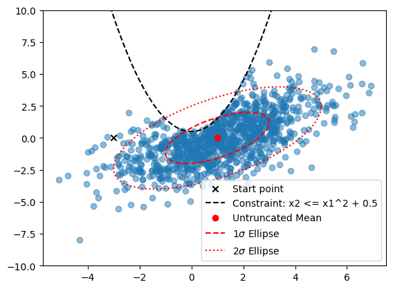
We sample from \(\mathcal{N}([1, 0]^\top, \Sigma)\) where \(\Sigma = 4\begin{pmatrix} 1 & 0.6 \\ 0.6 & 1 \end{pmatrix}\), constrained to \(x_2 \leq x_1^2 + 0.5\). The constraint is specified with:

\[\begin{split}A = \begin{pmatrix} 1 & 0 \\ 0 & 0 \end{pmatrix}, \quad \mathbf{f} = \begin{pmatrix} 0 \\ -1 \end{pmatrix}, \quad c = 0.5\end{split}\]

With \(\boldsymbol{\mu} = [1, 0]^\top\) and \(S = \Sigma^{1/2} \neq I\), the transformation is non-trivial:

\[\tilde{A} = SAS \neq 0\]

\[\begin{split}\tilde{\mathbf{f}} = 2SA\boldsymbol{\mu} + S\mathbf{f} = 2S\begin{pmatrix}1\\0\end{pmatrix} + S\begin{pmatrix}0\\-1\end{pmatrix} \neq \mathbf{0}\end{split}\]

\[\tilde{c} = \boldsymbol{\mu}^\top A\boldsymbol{\mu} + \mathbf{f}^\top\boldsymbol{\mu} + c = 1 + 0 + 0.5 = 1.5\]

Since both \(\tilde{A} \neq 0\) and \(\tilde{\mathbf{f}} \neq 0\), the sampler infers a QuadraticConstraint.

mu = np.array([1.0, 0.0]).reshape(-1, 1)
sigma = 4 * np.array([[1.0, 0.6], [0.6, 1.0]])
sampler = TMGSampler(mu, sigma, gpu=False)

# Constraint: x1^2 - x2 + 0.5 >= 0  =>  x2 <= x1^2 + 0.5
sampler.add_constraint(
    A=np.array([[1.0, 0], [0, 0]]),
    f=np.array([0, -1.0]),
    c=0.5,
    sparse=True,
    compiled=True,
)

x0 = np.array([-3.0, 0.0]).reshape(-1, 1)
samples = sampler.sample(x0, 1000, 100)

fig, ax = plt.subplots()
ax.scatter(samples[:, 0], samples[:, 1], alpha=0.5)
ax.scatter(x0[0], x0[1], color="k", marker="x", label="Start point")
x_vals = np.linspace(-5, 5, 200)
y_vals = x_vals**2 + 0.5
ax.plot(x_vals, y_vals, "k--", label="Constraint: x2 <= x1^2 + 0.5")
ax.scatter(mu[0], mu[1], color="red", label="Untruncated Mean")
theta = np.linspace(0, 2 * np.pi, 100)
ellipse = np.array(
    [
        mu
        + sp.linalg.cholesky(sigma).T @ np.array([np.cos(t), np.sin(t)]).reshape(-1, 1)
        for t in theta
    ]
)
ax.plot(
    ellipse[:, 0],
    ellipse[:, 1],
    color="red",
    linestyle="--",
    label=r"1$\sigma$ Ellipse",
)
ellipse2 = np.array(
    [
        mu
        + 2
        * sp.linalg.cholesky(sigma).T
        @ np.array([np.cos(t), np.sin(t)]).reshape(-1, 1)
        for t in theta
    ]
)
ax.plot(
    ellipse2[:, 0],
    ellipse2[:, 1],
    color="red",
    linestyle=":",
    label=r"2$\sigma$ Ellipse",
)
ax.legend()
plt.ylim([-10, 10])
plt.show()