Multiple Constraint Examples

This notebook demonstrates how to combine multiple constraints in tmg_hmc. Each call to add_constraint adds an independent constraint of the form:

\[\mathbf{x}^\top A \mathbf{x} + \mathbf{f}^\top \mathbf{x} + c \geq 0\]

When multiple constraints are present, the sampler requires all of them to be satisfied simultaneously, effectively truncating the Gaussian to the intersection of the constraint regions. Each constraint is handled independently during the HMC trajectory. The sampler detects which constraint boundary is hit first and reflects the momentum accordingly.

Setup

Install notebook dependencies if needed:

pip install tmg_hmc[examples]

from tmg_hmc import TMGSampler
import matplotlib.pyplot as plt
import numpy as np

# Set seed for reproducibility
np.random.seed(42)

Pinched Quadratic

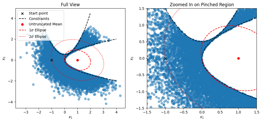
We sample from \(\mathcal{N}([1, 0]^\top, \Sigma)\) constrained to the region between two parabolas:

Constraint 1: \(x_2 \leq x_1^2 + 0.5\), specified as \(\mathbf{x}^\top A_1 \mathbf{x} + \mathbf{f}_1^\top \mathbf{x} + c_1 \geq 0\) with:

\[\begin{split}A_1 = \begin{pmatrix} 1 & 0 \\ 0 & 0 \end{pmatrix}, \quad \mathbf{f}_1 = \begin{pmatrix} 0 \\ -1 \end{pmatrix}, \quad c_1 = 0.5\end{split}\]

Constraint 2: \(x_1 \leq x_2^2\), specified with:

\[\begin{split}A_2 = \begin{pmatrix} 0 & 0 \\ 0 & 1 \end{pmatrix}, \quad \mathbf{f}_2 = \begin{pmatrix} -1 \\ 0 \end{pmatrix}, \quad c_2 = 0\end{split}\]

Both constraints have non-zero \(A\) and \(\mathbf{f}\), and the non-zero mean \(\boldsymbol{\mu} = [1, 0]^\top\) introduces additional linear terms after transformation, so both are inferred as QuadraticConstraints. The feasible region is the area below the first parabola and to the left of the second, creating a narrow, pinched region between the parabolas. To further illustrate the effect of the truncations, we plot the untruncated mean and 1 and 2 \(\sigma\) ellipsoids of the untruncated Gaussian in red.

This highlights one of the benefits of HMC style samplers, they are able to effectively mix even in tightly constrained regions like the pinched neck in this example.

mu = np.array([1, 0])
sigma = np.array([[1.0, -0.2], [-0.2, 1.0]])

sampler = TMGSampler(mu, sigma, gpu=False)

# Constraint 1: x1^2 - x2 + 0.5 >= 0  =>  x2 <= x1^2 + 0.5
sampler.add_constraint(
    A=np.array([[1.0, 0], [0, 0]]),
    f=np.array([0, -1.0]),
    c=0.5,
    sparse=True,
    compiled=True,
)

# Constraint 2: x2^2 - x1 >= 0  =>  x1 <= x2^2
sampler.add_constraint(
    A=np.array([[0, 0], [0, 1.0]]),
    f=np.array([-1.0, 0]),
    c=0,
    sparse=True,
    compiled=True,
)

# Initial point must satisfy both constraints:
# x2 = 0 <= (-1)^2 + 0.5 = 1.5 ✓  and  x1 = -1 <= 0^2 = 0 ✓
x0 = np.array([-1, 0]).reshape(-1, 1)
samples = sampler.sample(x0, 10000, 100)

# Compute 1-sigma and 2-sigma ellipses of the untruncated distribution
theta = np.linspace(0, 2 * np.pi, 100)
ellipse = np.array(
    [
        np.linalg.cholesky(sigma).T @ np.array([np.cos(t), np.sin(t)]).reshape(-1, 1)
        + mu.reshape(-1, 1)
        for t in theta
    ]
)
ellipse2 = np.array(
    [
        2
        * np.linalg.cholesky(sigma).T
        @ np.array([np.cos(t), np.sin(t)]).reshape(-1, 1)
        + mu.reshape(-1, 1)
        for t in theta
    ]
)

# Show two panels: full view and zoomed in to the feasible region
fig, axs = plt.subplots(1, 2, figsize=(12, 5))
x = np.linspace(-2, 2, 100)
for i, ax in enumerate(axs):
    ax.scatter(samples[:, 0], samples[:, 1], alpha=0.5)
    ax.scatter(x0[0], x0[1], color="k", marker="x", label="Start point")
    # Constraint boundaries
    ax.plot(x, x**2 + 0.5, color="black", linestyle="--", label="Constraints")
    ax.plot(x**2, x, color="black", linestyle="--")
    ax.scatter(mu[0], mu[1], color="red", label="Untruncated Mean")
    ax.plot(
        ellipse[:, 0],
        ellipse[:, 1],
        color="red",
        linestyle="--",
        label=r"1$\sigma$ Ellipse",
    )
    ax.plot(
        ellipse2[:, 0],
        ellipse2[:, 1],
        color="red",
        linestyle=":",
        label=r"2$\sigma$ Ellipse",
    )
    ax.set_xlabel("$x_1$")
    ax.set_ylabel("$x_2$")
axs[0].legend()
# Zoom in on the feasible region
axs[1].set_xlim(-1.5, 1.5)
axs[1].set_ylim(-1.5, 1.5)
axs[0].set_title("Full View")
axs[1].set_title("Zoomed In on Pinched Region")
plt.show()

Fully Constrained

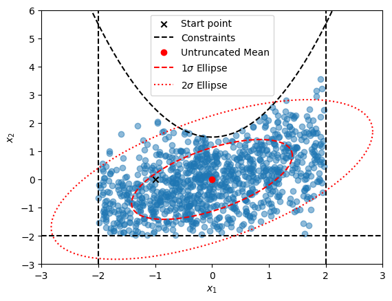
We sample from \(\mathcal{N}(\mathbf{0}, \Sigma)\) constrained by a mix of one quadratic and two linear constraints that together define a bounded, asymmetric feasible region:

Constraint 1: \(x_2 \leq x_1^2 + 1.5\) (quadratic upper boundary), specified with:

\[\begin{split}A_1 = \begin{pmatrix} 1 & 0 \\ 0 & 0 \end{pmatrix}, \quad \mathbf{f}_1 = \begin{pmatrix} 0 \\ -1 \end{pmatrix}, \quad c_1 = 1.5\end{split}\]

Constraint 2: \(|x_1| \leq 2\) (vertical bounds), specified with:

\[\begin{split}A_2 = -\begin{pmatrix} 1 & 0 \\ 0 & 0 \end{pmatrix}, \quad c_2 = 4\end{split}\]

Constraint 3: \(x_2 \geq -2\) (horizontal lower bound), specified with:

\[\begin{split}\mathbf{f}_3 = \begin{pmatrix} 0 \\ 1 \end{pmatrix}, \quad c_3 = 2\end{split}\]

Since \(\boldsymbol{\mu} = \mathbf{0}\) and \(S = \Sigma^{1/2}\), constraints 1 and 2 become QuadraticConstraint and SimpleQuadraticConstraint respectively in the transformed space, and constraint 3 becomes a LinearConstraint. This example illustrates how different constraint types can be combined freely.

mu = np.array([0.0, 0.0]).reshape(-1, 1)
sigma = 2 * np.array([[1.0, 0.6], [0.6, 1.0]])
sampler = TMGSampler(mu, sigma, gpu=False)

# Constraint 1: x1^2 - x2 + 1.5 >= 0  =>  x2 <= x1^2 + 1.5
sampler.add_constraint(
    A=np.array([[1.0, 0], [0, 0.0]]),
    f=np.array([0.0, -1.0]),
    c=1.5,
    sparse=True,
    compiled=True,
)

# Constraint 2: -x1^2 + 4 >= 0  =>  |x1| <= 2
sampler.add_constraint(A=-np.array([[1.0, 0], [0, 0]]), c=4, sparse=True, compiled=True)

# Constraint 3: x2 + 2 >= 0  =>  x2 >= -2
sampler.add_constraint(f=np.array([0.0, 1.0]), c=2, sparse=True, compiled=True)

# Initial point satisfies all three constraints:
# 0 <= (-1)^2 + 1.5 = 2.5 ✓  and  |-1| <= 2 ✓  and  0 >= -2 ✓
x0 = np.array([-1, 0]).reshape(-1, 1)
samples = sampler.sample(x0, 1000, 100)

# Compute 1-sigma and 2-sigma ellipses of the untruncated distribution
theta = np.linspace(0, 2 * np.pi, 100)
scale = np.linalg.cholesky(sigma)
ellipse = np.array(
    [scale @ np.array([np.cos(t), np.sin(t)]).reshape(-1, 1) + mu for t in theta]
)
ellipse2 = np.array(
    [2 * scale @ np.array([np.cos(t), np.sin(t)]).reshape(-1, 1) + mu for t in theta]
)

fig, ax = plt.subplots()
ax.scatter(samples[:, 0], samples[:, 1], alpha=0.5)
ax.scatter(x0[0], x0[1], color="k", marker="x", label="Start point")

# Plot all three constraint boundaries
x = np.linspace(-3, 6, 100)
ax.plot(x, x**2 + 1.5, color="black", linestyle="--", label="Constraints")  # parabola
ax.plot(2 * np.ones_like(x), x, color="black", linestyle="--")  # x1 = 2
ax.plot(-2 * np.ones_like(x), x, color="black", linestyle="--")  # x1 = -2
ax.plot(x, -2 * np.ones_like(x), color="black", linestyle="--")  # x2 = -2

ax.scatter(mu[0], mu[1], color="red", label="Untruncated Mean")
ax.plot(
    ellipse[:, 0],
    ellipse[:, 1],
    color="red",
    linestyle="--",
    label=r"1$\sigma$ Ellipse",
)
ax.plot(
    ellipse2[:, 0],
    ellipse2[:, 1],
    color="red",
    linestyle=":",
    label=r"2$\sigma$ Ellipse",
)
ax.set_xlabel("$x_1$")
ax.set_ylabel("$x_2$")
ax.legend()
ax.set_xlim(-3, 3)
ax.set_ylim(-3, 6)
plt.show()