Product Constraint Examples

This notebook demonstrates product constraints, a feature unique to exact HMC that allows sampling from regions defined by products of linear and quadratic constraints.

A product constraint has the form:

\[\prod_{i=1}^k \left( \mathbf{x}^\top A_i \mathbf{x} + \mathbf{f}_i^\top \mathbf{x} + c_i \right) \geq 0\]

Each factor is itself a linear or quadratic constraint. The product is satisfied when an even number of the individual factors are negative (or all are non-negative). This allows sampling from non-convex regions that cannot be expressed as a single quadratic constraint. HMC handles them naturally by computing the exact hit times for each factor and composing them into a product constraint.

Product constraints are added via add_product_constraint, which takes a list of parameter dictionaries, one per factor.

Setup

Install notebook dependencies if needed:

pip install tmg_hmc[examples]

from tmg_hmc import TMGSampler
import matplotlib.pyplot as plt
import numpy as np

# Set seed for reproducibility
np.random.seed(42)

Star Constraint

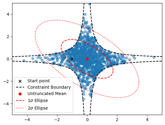
We sample from \(\mathcal{N}(\mathbf{0}, \Sigma)\) constrained to the region defined by:

\[(x_1 x_2 + 1)(-x_1 x_2 + 1) \geq 0\]

i.e. \(x_1 x_2 \in [-1, 1]\), which carves out a star-shaped region bounded by the hyperbolas \(x_1 x_2 = 1\) and \(x_1 x_2 = -1\).

Each factor is a simple quadratic constraint with no linear term (\(\mathbf{f} = 0\), \(\boldsymbol{\mu} = \mathbf{0}\)):

Factor 1: \(x_1 x_2 + 1 \geq 0\), specified with:

\[\begin{split}A_1 = \begin{pmatrix} 0 & 0.5 \\ 0.5 & 0 \end{pmatrix}, \quad c_1 = 1\end{split}\]

Factor 2: \(-x_1 x_2 + 1 \geq 0\), specified with:

\[\begin{split}A_2 = \begin{pmatrix} 0 & -0.5 \\ -0.5 & 0 \end{pmatrix}, \quad c_2 = 1\end{split}\]

Since \(\boldsymbol{\mu} = \mathbf{0}\) and \(S = \Sigma^{1/2}\), both factors become SimpleQuadraticConstraints in the transformed space (the non-identity covariance of \(\Sigma\) does not introduce linear terms since \(\boldsymbol{\mu} = \mathbf{0}\)). To further illustrate the effect of the truncations, we plot the untruncated mean and 1 and 2 \(\sigma\) ellipsoids of the untruncated Gaussian in red.

mu = np.array([0.0, 0.0]).reshape(-1, 1)
sigma = 3 * np.array([[1.0, -0.6], [-0.6, 1.0]])
sampler = TMGSampler(mu, sigma, gpu=False)

# Define the product constraint (x1*x2 + 1)(-x1*x2 + 1) >= 0
# This is satisfied when x1*x2 is in [-1, 1], carving out a star-shaped region
# Each factor is a SimpleQuadraticConstraint: x^T A x + c >= 0
parameters = [
    # Factor 1: x1*x2 + 1 >= 0  =>  A = [[0, 0.5], [0.5, 0]], c = 1
    {"A": np.array([[0, 0.5], [0.5, 0]]), "c": 1.0},
    # Factor 2: -x1*x2 + 1 >= 0  =>  A = [[0, -0.5], [-0.5, 0]], c = 1
    {"A": np.array([[0, -0.5], [-0.5, 0]]), "c": 1.0},
]
sampler.add_product_constraint(parameters=parameters)

# Initial point must satisfy the product constraint: x1*x2 = 0 which is in [-1, 1]
x0 = np.array([-1, 0]).reshape(-1, 1)
samples = sampler.sample(x0, 1000, 100)

# Compute 1-sigma and 2-sigma ellipses of the untruncated distribution
theta = np.linspace(0, 2 * np.pi, 100)
scale = np.linalg.cholesky(sigma)
ellipse = np.array(
    [scale @ np.array([np.cos(t), np.sin(t)]).reshape(-1, 1) + mu for t in theta]
)
ellipse2 = np.array(
    [2 * scale @ np.array([np.cos(t), np.sin(t)]).reshape(-1, 1) + mu for t in theta]
)

fig, ax = plt.subplots()
ax.scatter(samples[:, 0], samples[:, 1], alpha=0.5)
ax.scatter(x0[0], x0[1], color="k", marker="x", label="Start point")

# Plot the constraint boundary: hyperbolas x1*x2 = 1 and x1*x2 = -1
x = np.linspace(0, 5, 101)[1:]
ax.plot(x, 1.0 / x, color="black", linestyle="--", label="Constraint Boundary")
ax.plot(x, -1.0 / x, color="black", linestyle="--")
ax.plot(-x, 1.0 / x, color="black", linestyle="--")
ax.plot(-x, -1.0 / x, color="black", linestyle="--")

# Plot untruncated mean and covariance ellipses for reference
ax.scatter(mu[0], mu[1], color="red", label="Untruncated Mean")
ax.plot(
    ellipse[:, 0],
    ellipse[:, 1],
    color="red",
    linestyle="--",
    label=r"1$\sigma$ Ellipse",
)
ax.plot(
    ellipse2[:, 0],
    ellipse2[:, 1],
    color="red",
    linestyle=":",
    label=r"2$\sigma$ Ellipse",
)
ax.legend()
ax.set_xlim(-5, 5)
ax.set_ylim(-5, 5)
plt.show()